In previous posts, you have learnt how to add the developer tab to the excel file, how to navigate into the macro and how to clear the content. You can find these posts here.

Now it is time to learn how to run formulas in your Macro Excel VBA.

How to run formulas in Excel VBA

The main purpose of programming your own Macro tools,
it is to automate tasks that you perform on a certain frequency basis, independently of the size of the data.

While programming your macro,
you want to ensure your macro works no matter how many rows/columns of data there are in your file.  

Maximum number of rows and columns in excel

What is the maximum number of rows in Excel?
Every Excel file has a maximum of 1,048,576 rows, no more no less. 1,048,576

Which is the last column in Excel?
The last column in an Excel file is column XFD. XFD.

You may wonder why I would need such info… keep reading and you will find out!

Insert a formula in Excel VBA

This is what a formula in VBA code looks like:

Cells(row,column).Formula = "Formula"

Imagine you want to insert a vlookup in cell B2. How would you do it?

Cell B2 is the row: 2 and the column: 2 – thus we would be typing Cells(2,2)

Type your vlookup formula, and you would have your formula programmed in your Macro.

This is how your code would look like

Cells(2, 2).Formula = "=VLOOKUP(A2,'Data Countries'!A:B,2,0)"

How to autofill formula down to the last row of data in Excel VBA

While using the recording feature,
you run your formula in cell B2 and the following code gets generated.

    Range("B2").Select
    Selection.AutoFill Destination:=Range("B2:B10"), Type:=xlFillDefault
    Range("B2:B10").Select

The good news is that your code would work only when you have 10 rows of data.

The bad news is that your code would work only when you have 10 rows of data.
Imagine instead of 10 rows of data, you would have 250 rows of data,
how would you do it?

I get you covered here. Time to “Think like Excel”

To me, what I will show you down below is the best approach how to running formulas no matter the number of rows in your file.

Let’s see it with an example:

For the countries in column A, I want to include in column B the capital for each of the countries, using as reference the data set in the sheet: Data Countries

Step #1
All the data is in column A,
so we want to select the cell in the last row of this column – the column A
The last cell in the last row of column A is cell A1048576.
First, go to cell A10 and from that cell go to the cell  A1048576 (use the keyboard combination Ctrl +↓ and you will select cell A1048576)

If you want to do it using the Macro code – this is the VBA code to select cell A1048576:

Range("A1048576").Select

Step #2

Once the cell A1048576 is selected,  go all the way up (with keyboard combination Ctrl + ↑)
If you want to do it using Macro code – this is the VBA code to go all the way up:

Selection.End(xlUp).Select

What will happen when you go all the way up?
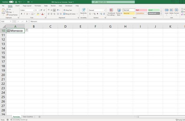
You will “hit” the last cell with data – in that case, the cell A10.

Step #3
Remember we are still “Thinking Like Excel”

As we want to run the formulas on column B, we will do an offset (0,1)
0 is the row and 1 the column.
While having selected the cell A10 and doing the offset (0,1)

We will be selecting cell B10

If you want to do it using Macro code – this is the VBA code to do an offset (0,1):

Selection.Offset(0, 1).Select

Step #4
Go up and run the formulas (with the keyboard you will need to perform two actions, one the action of going up Shift+Ctrl+↑ and two the action of running the formulas)

If you want to do it using Macro code – this is the VBA code to go up and run the formulas:

Range(Selection, Selection.End(xlUp)).Select
Selection.FillDown

Example of how to insert a formula in Excel VBA

Let’s see how to insert a formula in VBA with an example

Imagine I have one excel file with two excel sheets.

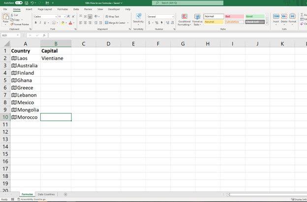
In sheet: Formulas I have 10 countries,
and for each country, I want to populate their capitals.

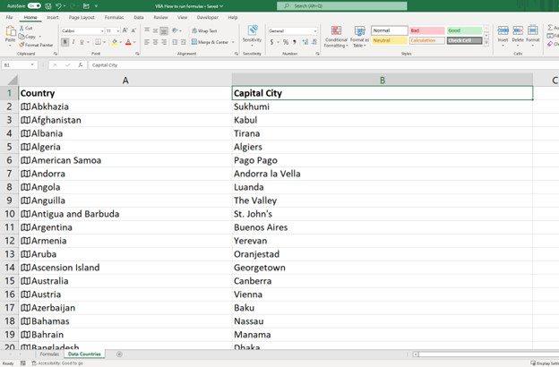
And in the sheet: Data Countries,
I have a database with all the countries in the world and their respective capitals.

Objective: show in Sheet Formulas the capital for each country

Step by step on how to do it without a Macro:

Step #1
In sheet: Formulas and cell B2 include a vlookup pointing to the Sheet: Data Countries

=VLOOKUP(A2,'Data Countries'!A:B,2,0)

Step #2
Select cell B10

Step #3 Select all the range – all the way up

You can do it with the key combination Shift + Ctrl + ↑

Step #4 Run formulas
Click on your keyboard the combination Ctrl + d

There it goes, you have the capitals of the 10 countries.

As a side comment for those 10 capitals, only one of those capitals has heating on the pavement,
you can even feel it while walking.
Could you guess which one? Hint: It is very cold there! 😀

Step by step on how to run a formula with a Macro:

Step #1 Type vlookup formula in cell B2

Cells(2, 2).Formula = "=VLOOKUP(A2,'Data Countries'!A:B,2,0)"

Step #2 Go to the last row in the file under the column A

Range("A1048576").Select

Step #3 Go all the way up

Selection.End(xlUp).Select

Step #4 Offset your position one cell by moving to the right

Selection.Offset(0, 1).Select

Step #5 Run the formulas and you will have your formula running as expected

Range(Selection, Selection.End(xlUp)).Select
Selection.FillDown

Full code ready to copy past into your VBA tool below:

Sub MisterPaton_formulas()
'Step #1 Type vlookup formula in cell B2
Cells(2, 2).Formula = "=VLOOKUP(A2,'Data Countries'!A:B,2,0)"
'Step #2 Go to last row in the file under the column A
Range("A1048576").Select
'Step #3 Go all the way up
Selection.End(xlUp).Select
'Step #4 Offset your position one cell by moving to the right
Selection.Offset(0, 1).Select
'Step #5 Run the formulas and you will have your formula running as expected
Range(Selection, Selection.End(xlUp)).Select
Selection.FillDown
End Sub

Reminder: Every macro needs to start with Sub and finish with End Sub
In this example – the macro starts with Sub MisterPaton_formulas().

Note: In this video, there is a mistake on purpose, if you notice it drop a comment below! 😀